3DM advanced: 3DM applied to GPCRs

Index

Note: Before doing this practice it is best to first do the practical on /wiki/spaces/DOC/pages/327684, which is the introduction to 3DM.

A: Introduction

Login at 3DM (app3dm.bio-prodict.nl) with your 3DM account. If you don't have a 3DM account you can request one via the "get 3DM" tab. To be able to do this course you need at least a course login. After you have requested an account you can request a course login by sending an email to joosten@bio-prodict.nl

Open the GPCR database at 3DM (app3dm.bio-prodict.nl).

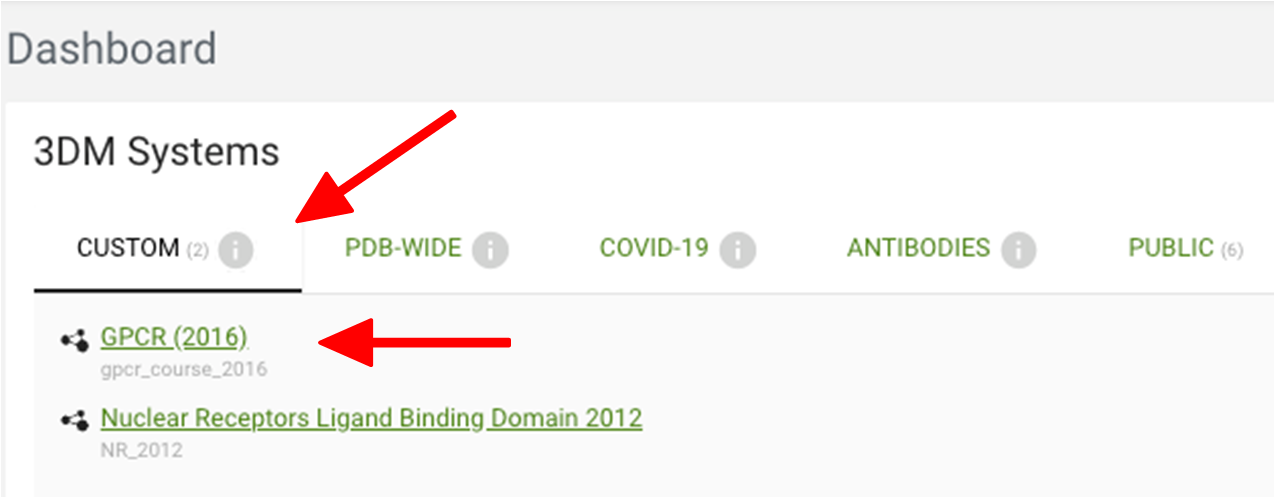
By default the GPCR 3DM database shows data of the GPCR family class A sequences. There are other classes of GPCRs too. You will investigate these later. Unless specifically requested otherwise, always use the GPCR class A protein family to answer the questions.

B: CorNet

Open 3DMs correlated mutation analysis tool CorNet by clicking on 'correlated mutations' in the left menu. You can see two big networks and a couple of small ones. You wonder if the two bigger networks really are two separate networks or if they are simply disconnected because of the fact that the default cut-off for the number of positions in the network is 25. Now answer the following questions:

Question 1

What does "independent networks" mean? When are two networks independent?

 Answer

If they are independent the residues in one of the networks mutate in sync with each other, but the residues from the other network mutate in a different rate. For example, If you compare two subfamilies the positions of one network all have a different residue in each of the two subfamilies (so they mutate between the two subfamilies), and the positions of the other network might be 100% conserved over the two subfamilies.

You can explore this idea by making an alignment with two groups of proteins. Each group should contain functionally similar proteins but this function differs between the groups. For instance, a group can be made with enzymes all converting the same substrate, and a second group that convert another substrate. The correlated mutations then often reveal hotspots that determine the substrate specificity change. A very important note is that correlated mutations reflect functional changes and not environmental changes. This can easily be explained: You cannot use correlated mutations to find hotspots for thermostability. You could make an alignment of two groups: one composed of proteins from thermophilic organisms and another made from non-thermophilic organisms. Then the differences between these groups should show up as correlated mutations, right? This is not the case, because in fact these two groups cover all sequences of the complete superfamily alignment. You can investigate the differences between these groups just by comparing the amino acid contents between the groups. This concept will be discussed later. One more important note: The problem with functional grouping is that the functional annotations of proteins is often based only on sequence similarity and can therefore be wrong. You need to make sure that at least a high percentage of the sequences share the same function to make functional based hotspot finding work. There are examples though were the alignment was successfully grouped simply by using keyword searches in the protein descriptions and used to find novel enzymes. The group of Prof Uwe Bornscheuer has found R-selective amine transferases (Only S-selective enzymes where known) by deleting from the protein family groups of proteins that had other activities based on motifs that were associated with the different functions. This exercise was repeated with 3DM. The protein family was first grouped by giving keywords that were related to enzymes with unwanted reaction mechanism. The keywords lyase, for instance, was used to select of enzymes with likely the unwanted lyase activity. Then, this set of sequences was used to find a sequence motif specific for lyase activity. All sequences that had this lyase specific sequence motif were subsequently deleted from the alignment. This step ensures that all lyases that were not annotated as such still get deleted from the alignment. This procedure was repeated for all different unwanted enzyme activities. This exercise resulted in 42 sequences that most likely are all R-selective amine transferases.


Question 2

How can you investigate if these two networks truly are two independently co-evolving networks? Don't do it yourself yet. Just think about how you would do this.

 Answer

There are multiple ways of doing this. One easy way would be to look at the amino acids distributions in each network. If the number of different motifs/different groups in each network differ (e.g. the positions of the first network all have only two different residue types and the positions of the other network all have five different residues) you know the two networks independently mutate. See question 6. Structural separation of the two networks might give a clue too.


Question 3

Give the Keyword "specificity" in the searchbox of the literature & mutations window on the right. What do you find? Gives this a clue about the separation of the two networks?

 Answer

Yes, one network clearly contains hotspots for specificity. This means that changes in specificity where the driving evolutionary force behind the correlated mutation behavior of this sub-network. For the other network there is no literature in the 3DM database describing mutations effecting specificity. As this database contains huge amounts of mutation data it is unlikely that these positions are hotspots for specificity.


Question 4

Do you think it is likely that position 92 or 93 have an important role for specificity? How would you find out?

 Answer

Yes, it is very likely they are also important for specificity. You could have a look in the 3D structure to see if they are close to the other members of this network (and/or close to the ligand binding pocket). But the only way to really make sure is to make mutations in the lab and test the binding affinity of the ligand. In enzymes such mutations would have an effect on the Km but not so much on the Kcat. Such mutations typically indicate a hotspot for specificity. The Km on other substrates might improve at such positions.

Correlated mutations often divide the superfamily into several groups based on sequence motifs. Sometimes this is just a evolutionary separation (e.g bacterial sequences vs eukaryotes), but because 3DM uses superfamily alignments containing proteins with different functions the correlation often are a result of the changes between these different functional groups.

Question 5

Do you understand the difference between evolutionary grouping and grouping based on functional differences?

 Answer
Usually 3DM alignments are composed of sequences from organisms from the entire tree of live. If you would make a phylogenic tree of the whole alignment and you see that it nicely overlays the tree of live, then correlated mutations can reflect the different domains of the tree of live. But most of the time multiple sequences from the same organism are in a 3DM alignment and these sequences can sequentially be very different. They almost always have different functions. Because there are proteins with different functions in an alignment the different groups of the phylogenetic tree are function based. This means that proteins with the same function form the large groups/clusters in the tree instead of the different domains or kingdoms of the tree of live. These different groups in such alignments result in correlated mutations that reflect the functional changes during evolution. Note that you can have both types of differentiation in one alignment.


Question 6

Click on the main node of the two networks (e.g. position 88 and 74). Clicking on a node gives information about this position, such as the amino acid distributions. How many different residues do you see in the distribution pie if you click on position 88? And what about 74?

 Answer

The pie chart of position 74 shows that there are two residues (W and F) very abundant at this position. Note that the * in the pie chart indicates all residues that are less than 5% present in the alignment. The variability at position 88 is much higher. 8 different residue types are available in more than 5% of the sequences. The two networks clearly show different mutation rates. To get the exact distributions you can click on "open position info page" below the pie chart.


Question 7

Click on the other members of each network. Do you see a pattern? Why does this tell you that these are truly separate co-evolving networks?

 Answer

Yes, most positions in the network of 74 have only two types of residues. The positions of the other network all have many more. This clearly shows that these two networks are independently co-evolving.


Question 8

Select at the same time 105 and 197. You can do this by making a selection box around the two positions (or selecting them while holding the Ctrl key). Looking at the amino acid distribution pie chart, do you think they might form a salt-bridge? Check this by clicking on "selected nodes" in the "Visualize alignment position in structure" option.

 Answer

The amino acid distribution of these two positions indicates that it is possible that they form a salt-bridge. In a large portion of the sequences they have opposite charge indicating they might structurally be close to each other and being able to form a salt-bridge. On the other hand there are quite some sequences that have E-E. This might indicate that they don't form a salt-bridge. You can simply check this if you select both positions and then click on "selected nodes" below the pie chart.

Give again the keyword specificity in the search box and look at the enrichment-score (overall enrichment) below the search box.

Question 9

Is this a high/meaningful value? Is it what you expect thinking about what you see in the network or is something going wrong? You can click on the information icon if you don't know what the enrichment-score (E-score) is.

 Answer

The E-score is quite low. An E-score of 1 means that there is no enrichment for the specificity related mutations in the network (just as likely to find specificity mutations at a position in the network as a position outside the network). There is nothing wrong, however, because not all positions of the complete network are hotspots for specificity. Only one small sub-network seems specificity related and thus the E-score for the complete network is low.


Question 10

Now select all the nodes (so both the green and the light blue nodes) of the sub-network containing the light blue positions (e.g. specificity positions). What is the enrichment score of this selection?

 Answer

The E-score for the sub-network is 5.0 (make sure the correlation cut-off is still set on the default of 1). An E-score of 5.0 indicates that the chance that the positions in this sub-network are specificity hotspots is 5 times higher than random. Or better, the chance they are specificity hotspots is 5 times higher than other positions. In other words: because these positions are important for specificity there has been an evolutionary pressure at these positions that has resulted in the alignment in this correlated mutational behavior. This is why correlated mutations are often referred to as "co-evolution".

Note that different protein features (activity, dimerization, etc) can be the underlying cause of an evolutionary pressure that has resulted in correlated mutations. In 3DM we pre-calculate the E-scores of different protein features at different correlated mutation cut-offs. The resulting plot shows quickly which evolutionary pressure is behind a correlated mutation network.

Fig 1. This figure shows the E-scores of different keywords. These figures are always availabe below the CorNet network. At high correlated mutation cut-offs specificity mutations are clearly over-represented in the GPCR CorNet network.


Question 11

Just below the search box there is the Keyword cut-off option. Set this on 1 and repeat the "specificity" keyword search. What does this option do? Why do you think 3DM has this value on 2 as default?

 Answer

If set on 2 then 3DM will only show positions in the network for which at least two different mutations have been published that had an effect on specificity. This is to ensure no false positives are included. In protein families for which a lot of mutations are available it is usually smart to leave this at at least two. If there is not so much data available it might be better to set it on 1 to get reliable E-scores.


Question 12

You can see that there is only one article describing a mutation having effects on specificity at position 93. Do think that it is likely to be a false positive or is it more likely that this really is a specificity related position? And what about position 248?

 Answer

As position 93 is part of the sub-network that has a high E-score for specificity it is very likely that 93 also is a hotspot for specificity. For position 248 on the other hand this is less clear. Note that 3DM "just" gives you the data. To make sure, always read the article. Especially if there is only one article found for a position.

Now select the other big network and color the nodes blue with the "node coloring" option that appears when you select positions in the window on the right. Select 247,248 and make them yellow. Select 42 and 32 and make them Magenta. Select position 60 (the only position of the sub-network that is not light bleu yet) and make it red. Click on "all nodes" in the "Visualize alignment position in structure" option. A new window will open where you can select structures to visualize the data. 3DM selects by default one structure. Just leave it as it is and click on either "visualize selection in Yasara" or "visualize selection in Pymol" depending on which program you have installed on your computer.

Question 13

Do the nodes of the specificity related network cluster together in the structure? How about the other big cluster?

 Answer

The specificity related network does cluster in the structure. The other big network doesn't cluster structurally and the function remains unclear based on structural data.


Question 14

Do you think that position 60 really belongs to the specificity related network?

 Answer

Considering the 3D location (near the ligand binding pocket and close to the specificity related network) position 60 probably is also a hotspot for specificity.


Question 15

What about the small separate network 247 and 248 for which we found one article describing effects on specificity. Might they actually belong to the specificity related network? And what about the other two small networks (e.g 32-42 and 153-251). Do you think they are related to the bigger network too?

 Answer

Just like 60, 247 and 248 are located close to the light blue positions of the specificity related network and are therefore likely specificity related positions. The role of the other residues are not clear based on this exercise.

If you use Yasara load the 1F88A co-crystalized compound using: 3DM → Structures → Load structure from 3DM and load the 1F88A drug. If you use Pymol start the 3DM plugin using "plugin → "initialize plugin system". Then "plugin" → "legacy plugins" → "3DM". A new window should start. Use your 3DM credentials to login and click in this window on 3DM menu → structures → load structures from 3DM, select 1F88A and only select "download drug".

Question 16

Do you think it makes sense to find the ligand there?

 Answer

There are several compounds crystalized in 1F88A. One of them is located inside the GPCR. This ligand is located exactly in between all the specificity related positions. This is a good example of how to use 3DM. With 3DM you are looking for correlations between different data types. In this case there is a good correlation between the CorNet network and structural location. If you find something like this your alarm bells should start ringing. In this case this screams specificity. If correlated mutations are located around the ligand (or substrate in case of enzymes) they almost always are specificity hotspots. Other examples of correlation between different data are: 

  1. High B-factor & High RMSD → hotspots for thermostability
  2. Motifs & sequence groups. For example: A sequence motif that is highly conserved in a subset composed of sequences with the same function and a different, again conserved, motif is found in a subgroup of sequences with another function. Often these positions determine the functional swap between the two subgroups (e.g. specificity hotspots)
  3. Ligand contacts & activity data of ligands. Some positions are bound only by inhibiting- or activating ligands → hotspots for inhibition and/or activation. A nice example was shown in the NR practical.
  4. Can you think of another example?

C: Families and numbering schemes

There are different families in the GPCR database. For each different GPCR class an alignment has been generated. These alignments are structure based and all have their own structural conserved core. Because these cores differ in length the different alignments have their own numbering schemes. Via the "Alignment" scroll down menu at the top of the 3DM website you can switch between the different families.

In the left menu, click on "System" → " System info" to open a nice overview of the different family alignments.


Question 17

How many aligned sequences do you see in the class A family?

 Answer

38,324


Question 18

How many sequences are in the different alignments?

 Answer

45,796 for the full alignment. 2,940 for class B, 3,978 for class C, and 4,008 for class F. Note that these numbers might be outdated when the database has been updated.


Question 19

Group A is by far the largest group of GPCRs. The "superfamily 3DM" is a combination of all the classes. Why do you think the superfamily 3DM is not as big as all groups in total?

 Answer

There can be different reasons. 3DM sometimes deletes sequences during the alignment generation procedure if they can't reliably be aligned. It might be that some sequences can reliably be aligned in the smaller family alignments because they have a bigger core. Meaning there are more residues that can be used to make the alignment resulting in more reliably aligned sequences. In the complete superfamily 3DM alignment only the trans-membrane helices are aligned (as those are the only parts that are structurally conserved between the different families). This means that there can be more uncertainty on the quality of the alignments. Another reason might be that some sequences are aligned in more then one class.

Now using the "alignment" scroll down menu select the superfamily 3DM and look at where the conserved residues are (which 3D numbers) using the "Alignment statistics" option from the left menu. Now do the same for the group A sequences (this you can do best in the other tab so you can switch between the tabs).

Question 20

What is the first residue that is conserved > 95% in the full alignment? What is it's 3D number in the full alignment? And in the class A alignment? Can you explain this?

 Answer

The first conserved residue (>95%) is Cys at position 68 in the full 3DM alignment. The same conserved Cys has number 81 in the class A family. There are less structural conserved positions if a structural conserved core is made for all the GPCRs. There are more positions structural conserved if only class A GPCRs are used to determine the structural conserved core.

Select from the "Numbering scheme" scroll-down menu at the top of 3DM the gpcr-A numbering in both alignments.

Question 21

Now compare the 3D numbers of the two conserved Cys residues again. What do you see? What is the number when using the class B numbering scheme?

 Answer

They have the same number using the class A numbering scheme: 3.25a. In the class B alignment this residue has number 3.29b. Obviously there are more structural conserved positions before this residue in the class B alignment compared to the class A alignment. When this common numbering scheme was designed they didn't realize that they could have made a numbering scheme that could be applied to all classes. As everyone uses this numbering scheme now, it is too late to synchronize the numbering schemes of the different families.


Realize that between different 3D alignments the 3D numbers cannot be compared (do you understand why you can't select gprc_a numbers if you have the GPCR class B alignment selected?). Because the size of the structural conserved cores differ between the different families different numbering schemes have been developed for the different subclasses. Each of these numbering schemes indicates for which subclass the numbering is. Although it could have been even better if they had used a common numbering for the transmembrane parts that is shared by all classes such that the conserved Cys would have had the same number in all classes. Even though this is not the case the commonly used numbering schemes designed for the GPCRs is a luxury that is only available in the GPCR protein family and has not been developed for any other protein family (as far as we know).

D: Making a structural model with 3DM

3DM contains an automated homology-modeling module. It uses the 3DM alignment between a sequence and a structure to generate models. At the protein detail page of a sequence you can find a model tab. Here you can select a suitable template to generate a homology model of the protein. 3DM already makes a pre-selection of suitable templates based on sequence similarity. You can choose any of the pre-selected ones. Which of these templates is best is for you to decide. This decision should be based on what you want to do with your model. For instance, enzymes can be in the open or closed conformation. If you want your model in the closed conformation, then start with a template that is in the closed conformation. Other factors can be: with or without ligand, with an activating/inhibiting ligand bound in the ligand binding pocket, etc. So, always first investigate the different starting templates to see which one fits best to your needs.

Hirschsprung disease is a disease that is caused by mutations in a GPCR.

Question 22

Using the "Literature" option of the "search" module try to find a human protein that is known to be involved in Hirschsprung disease.

 Answer

If you have searched in the titles of the articles you will find that there are two human proteins known to be involved in Hirschsprung disease: J7HDH6 and P24530.


Question 23

Go to the "protein detail page" of P24530. In 3DM you can simply click on the protein name. At this page you can see a "models" tab where you can create a structural model of a protein. Do you understand the different numbering options here?

 Answer

Alignment numbering: This uses the 3D numbers. Note that the active numbering scheme is used. This can also be a user defined numbering scheme. Later you will play with the different numbering schemes already available in the GPCR protein family. 
Residue numbering: This option uses the numbering of the sequence that is being modeled. 
Template numbering: This option uses the numbers of the template pdb structure.

Select a template and make a model. Make sure you have the GPCR class A alignment selected. Use Yasara or Pymol to open it. Making the model may take a few minutes. If 3DM wasn't able to model parts of the sequence, these parts will be missing in your model. These missing positions are indicated as purple dots in Yasara and as lines in Pymol. Usually this is because the alignment between the sequence and the template cannot reliably be made (often the parts outside the core) due to very low sequence similarities. Realize that those parts cannot be modeled reliably using the selected template, because the sequence similarity is so low that the two proteins will likely fold differently in those parts. Sometimes it helps making a model choosing a different template (if available), but usually this means that those parts can simply not be modeled reliably.


Question 24

Find positions where mutations can cause Hirschsprung disease using the "Literature hotspots" option of the 3DM menu in Yasara or Pymol. How many positions can you find?

 Answer

If you search with the keyword "Hirschsprung" with the literature cut-off set on 2 you will find that at 7 positions the literate reports Hirschsprung related mutations. In Pymol you can use the "Show scene content details" to get a list of the search results. Note that using "hirschsprung disease" as keyword doesn't change anything. But, sometimes you have to think about which keyword exactly to use to find what you need. For instance, if you search for mutations that resulted in a more active enzyme then you can use "increase activity" but also "high activity". The search works such that the words don't necessary have to be adjacent. So, a sentence like: "the A345Q mutant resulted in a enzyme of which the activity was increased", will also be found with the keyword "increase activity". If you put the literature cut-off on 1 you will see that there are many more positions mentioned in the literature in relation to Hirschsprung disease. 

Take home message: Always think about which keyword (combinations) and cut-off best to use.

E: Visualize data in structures

To visualize data in a structure you can use the "visualize" option. Here you can select multiple structures. All structures are superimposed. You can select one or more of the templates used to generate the alignment from, when "Show only templates" is selected from the quick filter menu. When activating the advanced setting, a PDB type can be selected. The "aligned" setting gives any of the other structures that could be superimposed on the templates can be selected. The "non-aligned" setting contains structures that were detected by BLAST but 3DM could not superimpose them on the templates. These structures usually are not belonging to the superfamily or are structurally too distantly related. Models you have generated with 3DM can be selected from the "model" setting. The name of a model indicates which protein is modeled and between brackets you see which structure was used to make the model. Do you see the one you made? From the "compounds" menu you can select any co-crystalized compound. These are also superimposed, so usually they will be in the pocket of the structures. You can select any combination of protein structure and ligand, so you can insert any ligand into any structure.

Question 25

Select a couple of structures and ligands. Then add positions, select the Correlated mutations tab and select the top five correlated mutations. From the "Conservation" select all residues >90% conserved. From the "Contacts" tab select all positions make at least 100 contacts with a ligand. Click on "visualize selection in Yasara" or "visualize selection in Pymol" and open the resulting file. Did you get back what you expected?

 Answer

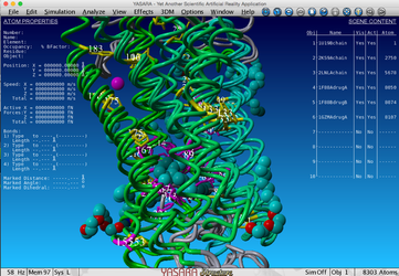
In this picture the first three templates were selected, the top five correlating positions, the first three ligands and all positions >90% conserved. You can see that the correlated mutation nicely surround the ligands located inside the GPCRs.

Click on "alignment statistics" in 3DM . Make sure you have the GPCR class A family selected and consult the "Human variation/Position" histogram. You can compare this histogram with other data types using the "compare with" option above the histogram. Choose here "Amino acid conservation". Set the cut-off for conservation on 50% and the SNP cut-off on 0,3.

Question 26

Do you find more SNPs at Conserved regions? Does this finding make any sense?

 Answer

SNPs are less common at conserved positions. With these cut-offs you see that the Enrichment is 0,55. These means SNPs are found less at conserved positions than at other positions. Note that it is important to set the cut-offs in this exercise because otherwise too many positions fall within the cut-offs to calculate a meaningful Enrichment-score.


Question 27

Now compare to ligand contacts. Do you see a common SNPs at a ligand contacting position?

 Answer

Not really. Maybe position 84. As SNPs are from genome sequencing projects of healthy humans you don't expect many SNPs at important positions as they might be damaging to the functioning of the GPCR, which, in turn, can result in a disease. This information can also be used the other way around. At positions where you find many SNPs it is likely that mutations are allowed. This means that they might be good candidates if you want to change the thermostability, because you can be quite sure that mutations won't harm the functioning of the protein.


Question 28

Reset the SNP graph by clicking "reset all". Move the cut-off to 1% using the slider bar and export the result to Yasara using the button left to the slider bar . Which positions were exported to the structure? Which of these very common SNPs is located near the ligand binding pocket?

 Answer

There are 7 positions: 29, 85, 130, 134, 145, 195, and 205. Position 85 is a common SNP closest to the ligand binding pocket.

Note that the  button can be found at many places in 3DM for direct visualization of data in Yasara.

F: Hotspot Baskets

There are other export buttons too, such as the "export to hotspot basket" button. Let's see how this works. Put the cut-off of the SNP graph again on 1 and open the hotspot basket tool by clicking on "HOTSPOTS" at the right corner of 3DM. At the SNP histogram this sign will appear: . This icon is for the insertion of selected positions in a hotspot basket. Then upload the 7 SNP positions into a new hotspot basket by clicking on the icon, give the basket a name, and save the basket.

Question 29

Go back to Yasara or Pymol and use the 3DM → Hotspot Baskets → Load a Hotspot Basket and open the basket you just created. In Pymol you need to define which hotspots you want to visualize from the basket. Simply select all 7. Is the result the same as you had before?

 Answer

The result should be the same.

A hotspot basket is nothing more than a selection of alignment positions. You can generate hotspots for different protein features (e.g. correlated mutations, specificity hotspots, thermostability hotspots, etc) and those can be found using 3DM. At a later stage you can open the basket in different 3DM tools. Let's see how this works.

Question 30

  • Go to the "correlated mutations" option in 3DM and use the keyword specificity in the "Literature & Mutation" window with a keyword cut-off of 1. Make sure you have the GPCR class A selected. Open the hotspot basket tool and select a NEW hotspot basket. Select the 9 positions of the sub-network that contains mutations reported to effect specificity upon mutation. Click on the "add to hotspots" buttonto store these specificity related mutations in a NEW basket. Give it a logical name and save it. We will use it later on.
 Answer

If all OK, you should have these positions in your basket: 84 88 92 93 98 109 218 245 248

A good trick for increasing thermostability of proteins is to make mutations at flexible regions. Go to the "Alignment Statistics" module of 3DM. Here you will find two histograms that display flexible positions. The RMSD (a measure for how tight the structures superimposed) and the average B-factor. The B-factor is a measure for how sharp the X-ray diffraction was for the atoms of a residue. A very sharp X-ray indicates that the amino acid is tightly positioned in the structure. The average B-factor is the average over all amino acids from all structures at an alignment position. Often these two plots show a similar pattern. If at a position both plots are high usually this is a good hotspot for changing thermostability.

Question 31

Make sure you have the hotspot basket window open. Increase the B-factor cut-off using the slider bar until you have <20 positions selected and store these in a new basket. Open Yasara or Pymol and open this basket in any GPCR you prefer. Does the result make any sense? Do you think these are positions that are likely good candidates to improve thermostability of GPCRs or is there an artifact in the B-factor method in GPCRs? Can you think of a way to solve this? Use the "literature hotspot" option (keyword thermostability) in Yasara or Pymol to find mutations from the literature that have an effect on thermostability. Do these overlap with the B-factor hotspots? Do you think this is a better way of finding hotspots for thermostability in this protein family? Right click on some of these positions and choose "3DM" → "amino acid distribution". Do any of these positions have a different residue than the consensus? Would it be smart to make the consensus if you want to increase thermostability? Is there a way of checking which mutations might be beneficial?

 Answer

The B-factor method doesn't seem to be a good method for the GPCRs. Likely this is because the transmembrane helices are so tightly bound that automatically the rest of the protein is much more flexible. It is known that making mutations in the transmembrane helices can make GPCRs more stable. This is nicely demonstrated by the "thermostability" literature search. Clearly the two methods do not overlap indicating that the B-factor method does not apply to GPCRs. It is in this protein family probably much better to first try the positions that are already published to have an effect on the stability. The best way to do this is to find amino acids described in literature that are known to stabilize GPCRs. If the stabilizing residue is not in your target GPCR then it might be a good idea to try that residue. If your target sequence has a different residue than the consensus it might be smart to try the consensus residue as there are several papers demonstrating that making the consensus often has a beneficial effect on the stability. (Note that if it is easy to screen your protein for thermostability than randomizing each hotspot might be smarter). There are many other tricks too. Here are some examples: 

  1. Introducing prolines at positions where a proline is common and your target doesn't have a proline
  2. Inserting negative charges at the N side of a helix (if there isn't any). Or a positive residue at the C-side. This is known as helix capping because the N terminus of a helix is slightly positive and the C-terminus is slightly negative.
  3. Creating salt-bridges by inserting positive or negative residues at positions on the outside of the protein. Always check if the residue you want to use is actually common in the alignment at that position.
  4. Replacing glycines where, according to the alignment, glycines can be replaced by something else.

G: Panel design

The idea of the panel design tool is to select sequences from the alignment such that the selected sequences are maximally distributed over the superfamily. This is done in two steps: First the sequences of the superfamily are grouped. This can simply be based on sequence similarity (similar sequences are within the same group), but groups can also be based on sequence motifs found at user selected positions. The last option is used to group sequences based on a protein feature. For instance, the user can pick positions important for specificity. The idea is that sequences that have the exact same residues (the same motif) at those positions they are likely to have the same specificity. Both methods can be combined. In the second step a user defined number of sequences (usually one or two) are selected from each group. The selection step contains all kinds of options to maximize the chance that these proteins are likely to express. Let's see how it works. 

Select the "panel design" option in 3DM. First we will divide the super-family based on sequence motifs. Because we want maximize the specificity range in the panel, we will use the "specificity hotspot" basket you have generated in question 30. This way all sequences with the same motif at our specificity hotspots (thus will likely have the same specificity) will be in one group. Use the "add hotspots" button to select the hotspot basket you made in Q30 (it should contain 9 positions).

Once they are selected click on "show groups".

Question 32

Based on these criteria, into how many groups is the alignment divided?

 Answer

1267 groups.


Question 33

By default the tool only selects groups with at least two members and deletes sequences that have a gap in one the selected positions. Do you understand the difference between "motifs" and "total groups"?

 Answer

Motifs for which only one sequence is available are not put in a group. The hypothesis behind this is that those might be sequence errors. Also sequences that have a gap at a selected position are not grouped. If you put "minimum group size" on 1 and deselect "hide motifs with gaps" the number of motifs is equal to the number of groups.

You can also divide the alignment phylogenetically. This separation can be combined to the motif grouping. In the box under "phylogenetic groups" you can give a number. The superfamily will then be divided into this number of groups purely based on phylogenetic distances. Reload the panel design tool (refresh the page) and type 10 in the box and click again on "show groups".

Question 34

How many groups are added by this exercise?

 Answer

There are now 1436 total groups.

After defining the groups you have to select from each group the sequences you want in the panel. There are several selection options that can be used to pick sequences from each group. First you select to number of sequences per group with the "proteins per group" option. Then several options can be used to determine which sequences are selected. These options are there to maximize the chance that selected sequences can be expressed. If there is literature available for a sequence, for instance, or if there is a structure available, then the chance that this protein can be expressed is higher since someone else has done it before. The different selection options can be combined using a "must have" or a "prefer" options. "must have" will result in a smaller number of groups, because not all groups will have a structure available, for instance. Usually it is a good idea to start with a larger number of groups that you want to have in your panel and delete some groups with these different options. Now play with the different options and see if you understand the result. To see the effect that the different options have you have to click on "select proteins". Any surprises? Can you make a panel of approximately 96 sequences for which you require swiss-prott, literature- and structure available.

Note that you can make the total panel smaller by clicking the "panel size" option. This will remove sequences by ensuring maximum diversity in the remaining panel sequences.


Note that sometimes you need to make a panel of a subset of sequences. For instance, say you want to find the most active enzyme with a certain specificity. Then you should first make a subset that contains only sequences that have this specificity. This sounds simple, but due to wrong notation of proteins is tricky. The best way to do this is to first do a keyword search to find enzymes likely to have the correct specificity and make a subset of this set of sequences. Then use this subset to make a motif with 4 to 7 amino acids that is specific for this subset. It is best to use the "subset specific residues" plot (consult the OAH questions about this plot). Make a new subset that contains all sequences that have this motif. With this approach you will not only find sequences with the correct specificity but that are annotated as "hypothetical protein", but you will also delete the sequences which are wrongly annotated. This approach doesn't make sure you have all sequences with the correct specificity, but it does maximise the chance that the ones that are in your subset all indeed have the correct specificity.

H: Literature on thermostability

Select "Alignment statistics" on the left of 3DM and scroll down to the "keyword mutation" histogram. Use the keyword "thermostable". You will find 24 positions that are related to this keyword. Open the hotspot basket tool and insert these 24 positions in a new hotspot basket, give it the name "thermostable" and save it. You will use it later.

At position 30 there is one thermostable mutation found in the literature. You can click on the bar at position 30 in the histogram. This will link to a page showing the corresponding paper. From here you can download the paper if you have access. If you don't have access you can also find the paper here.


Question 35

Can you find back the mutation at position 30? Is R the most common residue there, or can you easily mutate the R to something else based on the amino acid distribution. What is the most common residue at this position? Would Y be the first residue to try?

 Answer

In the abstract you can find R124. This R is at position 30. Remember that articles, of course, do not use the 3D numbers. In 3DM you can see which number is used in the article. If you go back to the 3DM page that gave the link to the paper you see that at position 30 mutation R124Y has been found. Remember the residue number when you go reading a paper. This makes it easy to find back the residue in the paper. Clearly this is a highly variable position and likely you can mutate this residue without destroying the function too much. Furthermore, R is not a very common residue. Even more "evidence" that the R can be mutated to something else. There is literature available that making the consensus often has a positive effect on the stability of proteins. Although we don't see this as a very common rule, in this case we do see that mutating to the most common residue has a positive effect on the stability.

The R124Y mutation is in the human Endothelin type B receptor (EDNRB_HUMAN).


Question 36

Can you find a structure of this protein in 3DM?

 Answer
  • Go to the protein detail page of P24530, make a model of this sequence and open it in Yasara or Pymol. Remember you can find a generated model at the "Visualize" option of 3DM.
  • In Yasara: look at R124 → use F3 to see all the atoms. Make the R124Y mutation (right click residue → swap → residue).
  • In Pymol follow the following steps:
    • Click on the ‘H' next to object in the object list. Select "Everything". The molecule will disappear.
    • Click on the ‘S' next to the object. Select "Lines". The structure will reappear with individual atoms visible.
    • In the top menu, click one Wizard > Mutagenesis. Click on the residue you wish to mutate.
    • In the Mutagenesis menu in the bottom right, click on the first button, which will normally say "No change". Here you can select the residue you wish to mutate to and click "Done".
  • Do you understand why this mutation might be stabilizing? Investigate all other mutations that are described in the abstract of the paper. Look at conservation and structural location to see if you would have picked these positions/mutations in order to change thermostability.


Question 37

Go to the protein detail page of P24530, make a model of this sequence and open it in Yasara. Look at R124 → use F3 to see all the atoms. Make the R124Y mutation (right click residue → swap → residue). Do you understand why this mutation might be stabilizing? Investigate all other mutations that are described in the abstract of the paper. Look at conservation and structural location to see if you would have picked these positions/mutations in order to change thermostability.

 Answer

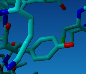
It is almost always very difficult by simply looking at a structure to explain the effect of a mutation. It is even more difficult to predict the effect by just looking in a structure. This is why it is so handy to have the 3DM data behind the structure. But let's just give it a try:

R124 (3D number 30) might be a bit more unstable because there is another positive residue (K34) very close to R30. K34 is actually really been pushed away from R30. The mutation to the Y makes it more stable. Also because the hydrophobic part of K34 nicely packs to the hydrophobic ring of Y30 (see figure).

D154 is not part of the core and doesn't have a 3D number. You can find this residue by looking in 3DM what 3D number residues have before or after this residue. 3D number Ile61 comes after the D154. Looking in the model you will find that D154 could not be modeled because the template doesn't have this residue. This could be solved by finding a template that does have a residue there, but 3DM cannot do this automatically and is therefore beyond the scope of this course. If you are interested in how to do this, find a good homology modeling course.

K270 (in 3DM: K163). This position is also highly variable. Although Ala is not the most common residue clearly the hydrophobic residues are by far the most common type of residue. So based on the amino acid distribution data mutating this Lysine seems a smart choice. Looking in the structure K163 doesn't really fit there and it is close to other positively charged amino acids. It's looks like mutating it to something hydrophobic will indeed have a positive effect on the stability and a smaller residue might fit there better as the side chain of K163 bumps into the side chain of L225.

S342A (3D number S220): This position is again highly variable. S in not very common at this position and just like K270 the larger hydrophobic residues are the most common residues. So mutating this residue seems a logical choice if you want to target thermostability. Looking in the structure there is not clear reason why Ala would be more stable than Ser.

I381A (3D: I250): This position contains mainly large hydrophobic residues. So mutating to Ala doesn't seem the best choice unless in our model the Ile doesn't really fit in the structure. Looking in the structure this is not the case. So why the I250A mutation is beneficial to the stability is unclear based on just these analyses.

Note that it is still very difficult to predict which mutations are beneficial for the stability of the protein. The best way to approach this problem is to find positions that are very variable because here you can make mutations without destroying the function. I seems a good strategy to target positions that have an uncommon residue and mutate those to more common residues.

I: Patent analysis tool

3DM contains an advanced tool for the analysis of patent data for complete protein families. How the tool works is explained in the Patent analysis presentation. Just go through the slides and then try out the tool yourself in the GPCR protein family via the "patents" option in the 3DM menu. 

3DM also contains a tool for analyzing patent data in a target sequence. You upload a target sequence to 3DM via system → custom proteins → add custom protein

J: Designing mutation experiments with the de-convolution tool

The de-convolution tool is a protein-engineering tool that is made for designing mutation experiments for a specific target sequence. With this tool many positions can be targeted at once without having to screen a large number of clones. The results of the measurements can be uploaded to the system and the system will calculate which mutations have the biggest effect on the feature(s) (e.g. activity or thermostability). The positive mutations can be combined to make the best performing sequence that can subsequently be used for a next round of engineering. Let's see how the tool works.

Go to Genomes (genomes.bio-prodict.nl) and login with these details:

  • Login: course_demo@bio-prodict.nl
  • Password: K7XlQAK23QvE8Bl%1i^L5#Ax460lC3

Once logged in you will see that we have set-up the de-convolution tool for one GPCR protein (P07550). At the right top you see an Erlenmeyer flask.

  • Click on the Erlenmeyer to open the tool
  • Click on "create new project"
  • Give the project a name
  • Select the target protein as the template of this protein engineering experiment
  • Create the project
  • Click on this project once it is available (sometimes the page needs a refresh to make it visible)
  • Click on "add round" to start designing the first round of mutations
  • Give it the name "round 1" and save it
  • Select "use the round 0 starting sequence (Note that if you already have uploaded experiment data in a previous round, you can use a sequence from that round)
  • Click on "save base sequence"
  • Now we can select mutations to introduce to the sequence. Click on "Mutations" on the left
  • We will use the hotspot basket generated previously. Select the "hotspots" tab and select the "thermostable" basket.
  • Click on "select all" to select all positions and select "Add all with most frequent as variant type" This option ensures that each hotspot is mutated to the most common amino acid according to the alignment. If the target sequence already has the most common amino acid it selects the second most common residue.

Note that the left box is a tool for the selection of mutations. Once you have the desired mutations you can drag them into the box on the right. Now the system automatically generated the mutations for all of the hotspots based on amino acid occurrences, but you can also manually add mutations.

  • Select the "Manual" tab in the left box and type V117C. To add this mutation to the experiment, simply drag this mutation into the right box.
  • Save the mutations by clicking "save" in the right box.
  • Click on "Sequences" on the left.
  • At "Maximum # of mutations per sequence" select 4 and select "fill up each sequence to contain maximum # of mutations". This will ensure that all sequences will have 4 mutations. If you don't use this option then sequences can have single, double, and triple mutations. Be sure to check the option “create demo measurement data”.
  • Select 96 sequences to generate and set the minimum number of observations to 2 and click on "convolute mutations".

This convolution step calculates the best sequences to measure. The tool maximally distributes the mutations over the 96 sequences. In real life the 96 sequences are ordered at a gene synthesis company and the thermostability of these 96 clones are then measured in the lab. These measurements must be stored in an excel file which can be uploaded to the system. You can download the template of this file at the bottom of the sequence list (export CSV). In this file you should enter the measured values and then upload the file via the "measurements" option on the left.

Because you are doing the course and we, of course, cannot ask you to make the measurements in the lab we generate random measurement values for your 96 constructs and you can right away jump to the "analysis" option on the left.

  • Click on "analysis".

To calculate the contributions of each mutation to the observed thermostability, click on 'Deconvolute measurements'. When done, the results will appear in a chart. There is a lot of information in these charts, but for now, let's keep it simple. In the top chart, unselect all colored boxes except the 'lm: single mutations" option. This will leave only the contributions calculated from a simple linear model visible. For more details about the various models available, see box 1.


Question 38

What is the best performing mutation?

Are there mutations that have a destabilising effect?


 Answer

The 'measured data' is randomly generated, so the best and worst performing mutations will be slightly different for everybody.


  • clicking on the point in the chart will cause a box with details about that mutation to load on the right side of the chart.
  • select the top-performing mutations. You can do this by dragging a box around them in the chart. Note that the selected mutations appear below the chart as 'selected mutations'. Click on 'add to selection'. This makes the selected mutations available for further use. After clicking, they end up in a box on the right of the chart. Here you can visualise them in the structure. Select a structure and make a visualisation and review it in yasara.
  • structure visualisations combined with detailed information about individual variants allow you to get a very thorough understanding about what might be happening in your protein.


Let's build a novel round.

  • in the left bar, add a novel round by clicking on the 'add round' link.
  • give your round a nice name and click on 'Create round'.

Now you would like to use a different base sequence than what you used in the first round. It makes sense to pick the best performing sequence from the previous round as the starting point for the new round. Let's do that.

  • click 'Select the best performing sequence from a previous Round based on a metric', select the first round and pick the thermostability metric.
  • then, hit the 'save base sequence' button below

Now it is time to pick the mutations that you want to test in the next round.

  • click on 'mutations' in the bar on the left.
  • click on the 'selections' tab

Here you can see the mutations that you selected in the previous round. These were the best performing mutations from your previous round. It makes sense to include them in this round.

  • click on 'add all' to move them to the right.


Question 39

You might see warnings like this: 'wildtype of mutation M279V did not match round base sequence'. How can this happen?


 Answer

Your base sequence will contain some mutations from previous rounds and in this case, there's a 'V' at position 279.


Your list of mutations for the next round is not complete yet. What you would do now in a real life scenario is to use all the insights you gained by analysing the mutations you previously made to select novel ones. Which positions worked, which didn't, etc. When your set of mutations is complete, you'd generate novel sequences, measure them in the lab, analyse the individual contributions and build novel rounds. Iterate you way towards a great protein!


Box 1. Detailed descriptions of the statistical models used in ‘classic’ deconvolution


Linear model: single mutations

The simplest model available is the linear model that takes into account only single mutations. This is a very straightforward model, basically just one formula in the form of:

EffectSize = a * mutation1 + b * mutation2 + c * mutation3 + ...

Given all the measurements (effect sizes) the numbers a,b,care optimised so that the final formula approaches the actual measured values best. The numbers a,b,c. are what you see in the deconvolution chart.


Glmnet: single mutations

This is basically a little smarter version of the linear model described above. What this model tries to do is the same as the linear model, but it tries to throw out all the parameters (or, mutations) that minimally affect the models performance. This model will usually consist of less mutations, and that is because it has thrown away mutations it deemed unnecessary. So, without those mutations, the model is still able to predict the actual measurements.

Same as with the linear model, the numbers a,b,c ... are what you see in the deconvolution chart.


Random forest regressor: single mutations

This is the least interpretable of the models I guess. The predictive model that tries to predict the measured values based on the mutations present in the sequences is a random forest model. This model consists of a number of 'decision trees' that are optimised to predict the measure value. A tree is basically a series of decisions, like "if mutation1 is present, but not mutation2 , predict measurement value x". The good thing about this is that interactions between mutations are inherently taken into account. The values that you see in the deconvolution chart are derived from the number of times a

mutation is used in a "split" in the tree, together with the position of the split in the tree, where higher-up splits are more important.


Then there are a number of models that include only interactions, or interactions combined with single mutations. Interactions are terms in the models that basically 'group' multiple mutations as one term. So if you have a sequence where mutation1 and mutation2 are present, their interaction will be one term (e.g. mutation1+2 ). So in the case of a linear model you get something like

EffectSize = a * mutation1 + b * mutation2 + c * mutation3 + d * mutation1+2

this is an example of a model with both single mutations and interactions, but you can also do this of course with just the interaction terms.
The downside of including interactions is that you get a very large number of parameters and you tend to overfit very easily, which is why there is no linear model that includes interaction terms, but only glmnet ones.